Overview
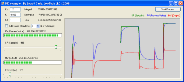
This code is a working example of a
PID
(Proportional, Integral, Derivative)
control.
This type of a
control
is used when
processes
change due to inertia. (A car's cruise
control is a
PID
controller.)
The PID
algorithm is surprisingly simple, and can be
implemented in five lines of code. There are three
constants that must be determined in order to shape
the control's
output. The three constants as well as the set point
and sampling interval can be changed in real time.
The resulting shape of the output will be displayed
in a strip chart.

How are PID loops
used?
Many real
world processes
build up over time.
When you step on the accelerator, your car moves
slowly, then faster, and faster still, until you let
off the gas pedal. As you speed up, you press the
gas pedal less, then a little less, then even less,
until you reach the speed limit. Unlike the digital
world where things are either “on” (1) or “off” (0),
real processes
have varying degrees of “on”. In the driving
example, how much the accelerator is turned “on”
depends on the car's current inertia and how
different the car's speed is from the speed limit.
Controlling
such a process
with inertia can be done with only five lines of
code. But, just like learning to drive, it takes
practice to know if you are starting too quickly, or
if you'll overshoot the speed limit.
Cruise
control
is one example of a PID
control loop.
To calculate the output, it needs three factors. The
first, (P), is the difference between the current
speed and the desired speed. The second, (I), is the
sum of the differences over time. And, the third,
(D), is the rate of change between sampled
differences. Each factor is scaled by a gain
constant; they are refered to as Kp, Ki, and Kd. The
value of these gain constants determines how
responsive the output will be. If the Kp, Ki, and Kd
values are too high, the output (car's speed) will
far exceed the set point (speed limit). Set too low,
the output may never reach the set point (like
driving 40mph on the highway).
Code implementation
In the real
world, a
process
updates constantly. In order to
simulate this
action, a timer is used to run an equation that
models the
process.
From a second timer, the
PID
control
algorithm samples the
process
value at a rate slower than the
process
model updates. The “Process
Value” or PV timer should run at least twice as
faster than the “PID
control”
timer. In the application, the PV timer runs every
17ms, and the PID
timer runs every 100ms.
The PV timer (tmrPV)
tick event handler runs the following code:
 Collapse
 |
Copy Code
private void tmrPV_Tick(object sender, EventArgs e)
{
PV = PV + (output * 0.20) - (PV * 0.10) + noise;
}
The PID
control
timer (tmrPID_Ctrl)
tick event handler runs:
 Collapse
 |
Copy Code
private void tmrPID_Ctrl_Tick(object sender, EventArgs e)
{
error = setpoint - PV;
integral = integral + (error * Dt);
derivative = (error - preError) / Dt;
output = (Kp * error) + (Ki * integral) + (Kd * derivative);
preError = error;
}
Take a look at some typical output shapes
In the images below, the green line is the set
point, the blue line is the input (or
process
value), and the red line is the output (or
manipulated value).
Correct
control
signal. All three gain constants are set
correctly.
Overshoot. Integral constant too high.
Undershoot. Integral constant too low.
Ringing. Integral and Proportional gain
constants too low.
Noise (under
control). All three constants are set
correctly.
Noise (not
controlled). Derivative gain constant too
high.
Code modifications
you might consider
This example works for modeling any
process
that has inertia. The
process
being modeled here is a car's cruise
control.
In order to adapt the code to model a
process
other than cruise
control, the equation in the PV timer tick
event handler should be changed.
I use PID
loops for electric furnace
control.
In furnace
control,
thermal mass is measured by sampling temperature.
Better PID loop
tuning results in efficient energy use. The code
currently in the PV timer tick event handler is
pretty close to a furnace equation. You can modify
the equation to fit the system you want to model. As
a rule of thumb, use the following equation:
 Collapse
 |
Copy Code
ProcessValue = ProcessValue + (output * efficiency) – loss
In a real cruise
control,
there are limits on how much the output can change
from sample to sample. This example does not include
any way to limit the output's magnitude of the
change. Such code might look like:
 Collapse
 |
Copy Code
if ( (output – outputLast) > maxChange)
  output = outputLast + maxChange;
else if ( (outputLast – output) > maxChange)
  output = outputLast – maxChange;
outputLast = output;
The noise that can be added to the signal is not
representative of anything your car might encounter.
(It is really just a model of electrical noise.)
Noise to a car's cruise
control
might be something like a hill, or a gust of wind.
Both of those examples have a lower frequency than
our noise. Since the noise is created in its own
timer event handler, you can change the interval of
the noise to change its frequency. You could also
change the noise equation to model the effects of a
hill, or even a chilling arctic blast.


